On The Intrinsic Knowledge Retrieval Scaling Challenge

Part I: The scaling problem inside every Knowledge Retrieval system

A large set of documents was added to your knowledge base last quarter. Nothing broke. The index built fine, latency held, the dashboards stayed green. But somewhere in there, questions that used to cite the right documents are now giving answers based on less ideal ones - they stopped retrieving the best documents. This is the quiet failure mode of retrieval at scale.

As RAG systems as well as agentic flows that heavily depend on knowledge retrieval move into production connecting to just about all of a company's corpus that may contain millions of documents, this is a substantial and important challenge to address.

We justify these points and test them in detail in a study using two very different corpora, EnterpriseRAG-Bench and BrowseComp-Plus.

In Part 2 of the blog series, we'll show some techniques how agentic retrieval can win back much of the recall that scale takes away, building directly on what's here.

Limitations and Assumptions

A few notes to start:

• The primary contribution here is synthesis and application: combining existing research and applying it to modern agentic/RAG questions around "adding to the corpus," worked out in detail for one specific corpus. The underlying pieces come from keyword-era IR, score-distribution statistics, the kernel two-sample test, recall-from-sampling work, and a few recent RAG papers - all cited in the References.

• We only explicitly test on a corpus combining data from two specific benchmarks and one embedding model, but we believe the core concepts to be universal.

• As we scale up the corpus for the most part we assume that the added documents are detractors, addressing the problem of the ‘correct’ information/document being washed out by new ones. In reality of course, scaling is a lot more complex and often the new set has better or newer information. We will provide a short discussion on how to estimate this from a sample but then focus again on the impact of distraction.

• By design, we consider straight, unmodified, single-shot semantic search (and to a lesser extent BM25) recall without answer generation, as these tend to be a core, atomic component of modern broader agentic retrieval approaches. Hence, understanding these and their failure modes are essential to understanding and improving complex agentic flows.

• The model and its shortcuts make assumptions. The math idealizes added documents as independent competitors, and the cheap, label-free screens we propose lean on mild assumptions about how a new source competes for your answers.

• The shapes our tests show are probably general; the magnitudes - how fast recall falls, where it bottoms out - are properties of your data and embedding model. The present work is a suggestion on how to evaluate your data.

---

1. "How many documents?" is the wrong question

The questions everyone asks are "what happens to my retrieval if I scale to a million documents?", "what happens if I connect more sources of substantial size", or "how does the data from a different part of the business affect my retrieval results". They feel like the right questions, but they are incomplete.

Intuitively, it is clear why that is: imagine a knowledge base full of cloud-infrastructure docs. Dump a hundred thousand documents about soccer games into it, and your search for "Kubernetes pod scheduling" doesn't get any worse - the soccer docs simply live in a completely different part of the space and never come up as candidates. Now instead dump in a hundred thousand more infrastructure docs. Suddenly the right answer is competing with a crowd of near-identical neighbors, and your recall drops.

Same number of documents. Very different outcomes. The variable that mattered wasn't how many you added - it was how much they resemble what you already had.

That reframing is critical and it leads to a more useful question:

As my corpus grows, how does my recall actually change - and can I predict that, and screen a new data source for damage, before I pay to index all of it?

One clarification heads off a real confusion. We're asking whether a specific document you already know is the best answer keeps getting retrieved as the corpus grows around it - treating every new document as a potential detractor.

That's a different question from "does a bigger corpus make my RAG answers better overall," where more documents can actually help by covering more answers (Ning et al., 2025). Both can be true at once; this post is largely about the first (although we will suggest a method to also estimate the second). Holding the right answer fixed, every document added is one more thing that can push it down the list - and with long-running agentic flows that also take action, the problem can compound.

---

2. The framework

The framework rests on two ideas: similarity decides which documents can hurt a question, and the k/N ratio decides how much. Only documents close enough to compete with a question's existing answer matter - everything else is effectively invisible - so what governs recall isn't so much corpus size as how many genuine competitors a question has.

Under representative growth (new documents drawn from the same distribution as the old), those competitors climb in step with the corpus, so an answer keeps its top-k slot as long as k/N holds: top 10 of 50,000 is about as hard as top 100 of 500,000. A far-off source stays far from your questions too, so it barely moves recall; a specific on-topic one drives it down faster. That growth erodes retrieval is long known — Hawking & Robertson showed it for keyword search in 2003 - and it carries cleanly to embeddings.

We build this up in two steps: first a single corpus growing by random samples, then a specific new source added to it.

2. 1. Growing a corpus homogeneously

2.1.1 Recall@k depends on k/N, not $k$ and $N$ individually

Give every question one number, its difficulty $p_q$ ​ - the probability that a randomly drawn document outscores its right answer. $p_q$ ​is a rate, not a count: a property of the question and the documents in the corpus, that is approximately fixed as the corpus grows homogeneously. Across $N$ documents the answer's rank (the position of the gold document in a search ranking) is then one (itself) plus however many beat it:

$$\mathrm{rank}(q) \sim 1 + \mathrm{Binomial}(N, p_q), \qquad \mathbb{E}[\mathrm{rank}(q)] \approx 1 + N p_q,$$

as $\mathbb{E}[\mathrm{Binomial}(N, p_q)] = N p_q$. It survives, in the average, the top $k$ if $p_q \lesssim k/N$, so with $F$ the distribution of difficulty across the questions, we have

$$\mathrm{recall@}k(N) = \Pr\left(p_q \lesssim \frac{k}{N}\right) = F\!\left(\frac{k}{N}\right).$$

Recall is the share of questions easy enough to clear the bar - and the bar is the ratio $k/N$, nothing else. Because difficulty doesn't move as $N$ grows - if the new documents are sufficiently similar to the existing ones - doubling the corpus costs exactly what doubling $k$ wins back. (Reading effectiveness of a score distribution this way is standard in IR and query-performance prediction - Manmatha et al., 2001; Kanoulas et al., 2010; Vlachou & Macdonald, 2024.)

2.1.2 The shape of the recall curve

Having established the k/N-dependence, we can ask what type of curve we can expect. As $N$ grows for a fixed k, $k/N$ decreases and we would expect recall to decrease or stay constant as the ranking of the gold doc can only worsen. An S-curve-type behavior is then likely expected, with a near-linear part in the middle: with $k>1$, as we increase document count from near-zero (say, only gold documents) and recall likely close to $1$, initially recall would very slowly decrease as new documents may push the gold documents down but most are still at a position < k. The decline in recall would then start to accelerate before, as it is capped at 0, would decelerate again and flatten out.

The natural x-axis for this process is $\log N$ (or $\log N - \log k$) rather than $N$ or $k/N$ — we are less concerned with how many documents are added, but by what factor we grow the corpus.

How large and steep is the near-linear part of the S-curve, where recall drops fastest and the system essentially goes from ‘good’ to ‘bad’? Is behavior falling off a cliff or is it a long gradual process?

The slope in natural log coordinates is:

$$\frac{d(\mathrm{recall})}{d(\ln N)} = -\frac{k}{N}\, f\!\left(k e^{-\ln(N)}\right) = -\frac{k}{N}\, f\!\left(\frac{k}{N}\right), \qquad f = F'.$$

where $'$ is the derivative with respect to $x = k/N$. (Note that this is constant if $F(x) \sim \ln(x)$). Since $F(x)$ is the fraction of questions that have the gold document within cutoff range $k$ at scale $N$, $f(x)$ is essentially the number of questions that change status at $x$ (per unit of $x$) divided by the total number of questions.

• The shape of the recall curve really depends on the difficulty distribution F(x) of the questions - there is no intrinsic shape built in outside of the constraints discussed earlier.
• If all of the questions are of very similar difficulty in the sense as defined above, F(x) will be constant as x decreases (N increases) until suddenly for the bulk of the questions the gold documents drop below cutoff $k$ and a sharp drop in recall occurs.
• If $F(x)$ has multiple modes (clusters of questions with similar difficulty), the recall curve will have multiple scales of steeper dropoffs.
• If $F(x) \sim \ln x$ along an extended range of $x$, recall drops linearly in that area, representing a more gradual impact. What does this condition mean intuitively? For a given corpus size, there would be just as many questions where the gold documents are ranked in the interval (5, 10] as for the interval (10, 20], etc.

While there is no guarantee that the last condition $F(x) \sim \ln x$ is obeyed by a given question/corpus pairing, we believe that it is quite natural and we would expect gradual decline in recall@k as $N$ scales up and the region over which the bulk of the drop in recall occurs tends to be rather extended.

2.1.3 Projecting behavior at scale from one measurements at small scale

A key takeaway from this discussion is that - thanks to the fact that $F= F(k/N)$ vs $F = F(k, N)$ - for homogeneous scaling, we can learn a lot about recall at large scale from measurements at small scale and lower $k$: Sweeping $k$ at a small size already traces the whole curve (up to a scale) - so for example recall@2 at scale $N_{\text{small}}$ should be very similar to recall@20 at scale $N_{\text{large}} = 10 \times N_{\text{small}}$. Since $k$ can't drop below 1, the smallest ratio you can measure at the small scale is $1/N_{\text{small}}$ - so this trick reaches up to a corpus of size $K \cdot N_{\text{small}}$, where $K$ is the cutoff you ultimately retrieve at (a scale-up factor of K). But even that bounded reach is very helpful: from a 5k sample swept down to $k=1$ you can already anticipate recall@100 at 500k. More sophisticated subsampling should be able to extend it further.

Note that this discussion does not depend on a particular smooth corpus. Since these are *direct count of real ranks* clusters and other real-world complications like near-duplicates are already baked in.

2.1.4 Application areas

Organic corpus growth should typically be reasonably uniform so the earlier discussion should apply to a good approximation. However, live corpus growth is also quite slow, so any change in behavior should be developing over time.

However, the formalism outlined above could also be used for POC-type situations for very large corpora - Indexing only 1-10% of the data can already be quite informative.

2.2 Adding documents that are not fully in-distribution

There are however many situations in real life in which the data to be added is not all that homogenous - new document sources may be added that may have a different format and focus, a new business unit may be added, or a completely new and unrelated set of data should be included in the system to provide the solutions benefits to more data.

And the impact of those changes would come fast.

In these situations we have the existing data, that we call corpus $A$ and we want to add new data, let’s call it corpus $B$. How can we make projections about B’s impact before indexing the potentially massive amount of new data?

2.2.1 Are corpora $A$ and $B$ close?

The cheap first check. From a sample of $B$, take the average cosine similarities within $A$ ($S_{AA}$), within $B$ ($S_{BB}$), and across the two ($S_{AB}$), and combine them into the maximum-mean-discrepancy statistic (Gretton et al., 2012):

$$\mathrm{MMD}^2(A, B) = S_{AA} + S_{BB} - 2\, S_{AB}.$$

This expression was derived as a statistical test to determine whether two samples likely come from the same distribution. (In fact, the S expressions can be more general, using general kernels vs cosine similarities).

In our context this should probably be read however more as a graded distance.

What does this mean?

• if $S_{BB} \sim S_{AA} \sim S_{AB}$ then the documents in $B$ occupy a similar region in the semantic space, and interference is quite likely;
• if on the other hand $S_{BB} \sim S_{AB}$ and $S_{AB} \ll S_{AA}$ then $B$'s documents are in the average far away from $A$'s — so it is probably safe to add.

We consider this a useful first test.

It is important to stress though this is a bulk statement or measure. Even if the test would suggest ‘probably safe’, a few ‘well-placed’ distractors can push out the correct answers, so a large $\mathrm{MMD}^2(A, B)$ is no proof that recall will not be affected.

If we want to go from the bulk statements to a more precise estimate whether B’s documents can interfere with A’s, we have to look at the actual neighborhoods of the questions. Fortunately, we can learn a lot by using samples of $B$.

2.2.2 Are B’s near to questions? If a test set is available: the competition discount

What we really would want to study is how close are the documents in $B$ to the questions compared to the ones in A. Let $a_q$ be the number of A-documents that already outrank its gold answer - just its current rank in A, minus one.

Then we can sample m documents from $B$ (which itself contains M documents) and measure $r_q$, the fraction of the sample that outranks that same answer. ($r_q$ is a rate, so its value doesn't depend on $m$ - a larger sample just pins it down more tightly.) Comparing it to the answer's difficulty in your own corpus, $p_q$, gives the competition discount

$$c_q = \frac{r_q}{p_q} \geq 0.$$

This ratio captures how much more (or less) likely documents from $B$ are to displace the gold document vs those from A.

As a simple estimate of the recall after adding the full M documents of B: the number of documents ahead of the gold answer climbs to $a_q + M \cdot r_q$. So the per-question forecast is simply:

$$\text{the answer survives in the top } k \text{ as long as } a_q + M \cdot r_q < k.$$

Of course, this is an estimate with high variability. Two points need to be made:

• Averaging the results should provide an unbiased estimate. However, substantial clustering may well create substantial variance. In our test in the next section we will show however that for the EnterpriseRAG dataset this does not seem to create a substantial problem.
• You will need a decent size test set to arrive at a reasonable estimate for the recall that includes $B$.

You can also replace each $a_q$ with the corpus average $N_A \cdot p_q$. Then, since $M \cdot r_q = c_q \cdot M \cdot p_q$, the competitor count factors to $(N_A + c_q \cdot M) \cdot p_q$. Treating the discount as a single representative value $c$ — the average of the $c_q$ across questions — the whole effect collapses to one line:

$$\textbf{adding } M \textbf{ documents of } B \approx \textbf{adding } c \cdot M \textbf{ documents of your own corpus } A$$

Note that you can then read the new recall with $B$ straight off the $k/N$ curve that you can measure from $A$ alone, at effective size $N_A + c \cdot M$.

The discount says how much each B-document counts: $c = 0$ is free ($B$ lives elsewhere in the space), $c = 1$ is "just more of $A$," and $c > 1$ means $B$ competes harder than your own corpus — its documents outrank your answers more often than $A$'s do, a source even more aligned with your questions than what you already have.

2.2.3 Estimates without a test set: how much worse than today?

What if you do not have a test set with gold documents? Can I still provide some estimate for ‘how much worse’ the system is likely to get?

If you have no labels you can still say and do a lot - using only your questions, your current corpus A, and a random sample of B:

Run each question against $A$ plus a sample of $B$ and look at your top $k$ as before. Count how many of those slots are now B-documents and estimate the expected number at full $B$ scale — call it $n_B$. That single count is the whole measurement, and it needs nothing but the question: every B-document that muscles into your top $k$ is one that shoved an A-document out, so your A-results have been squeezed into the top $k - n_B$. Your effective cutoff just slid from $k$ to $a^* = k - n_B$. On average, $\mathrm{recall}_{\text{new}}@k$ would then be reduced: $\mathrm{recall}_{\text{new}}@k = \mathrm{recall}_{\text{orig}}@(k - n_B)$. (Same variance caveats as before.)

2.3 What if the new documents are better?

Everything so far has treated $B$ as a pure detractor. But as Ning et al. (2025) note - and as you'd expect - more documents can also help by supplying an answer better than anything you had. With an LLM-as-judge standing in for the labels you don't have, you can estimate how often that happens, too. Here is a proposal for the procedure.

Run your questions against $A$, then against $A$ plus a sample of $B$. Dedupe the two result sets and hand each question's candidates to a properly prompted judge — but ask it to do slightly more than pick a winner: have it count, per question, how many of the sampled $B$-documents it rates above your best $A$-document. Call that count $b_q$ out of a sample of $m$, so a single $B$-document beats your best with rate $\hat{\pi}_q = b_q/m$.

The extrapolation isn't the additive one from the detractor side, because here you only need one better document - extra good ones don't help. So the probability that full-size $B$ improves a question saturates rather than stacking:

$$\Pr(B \text{ improves } q) = 1 - (1 - \pi_q)^M,$$

and aggregating this over the corpus we get:

$$w_B = \frac{1}{|Q|} \sum_q \left[1 - (1 - \pi_q)^M\right],$$

where $w_B$ is the average per-question likelihood that the new documents improve existing questions.

This number is not to be added or subtracted from the recall curve; it really measures a different dimension of the impact of scaling up.

---

3. An explicit scalability study

We tested this approach by using (and combining) two very different corpora, EnterpriseRAG-Bench, and BrowseComp-Plus.

EnterpriseRAG-Bench (eRAG), proposed in Sun et al (2026), is a synthetic corpus of ~510k documents simulating a fictional enterprise: emails, Slack messages, tickets, phone call transcripts, Google documents, etc. - all orbiting the same business domain. By its nature, it is semantically dense: the documents discuss overlapping topics, reference the same projects, products, and initiatives, and use similar vocabulary. The benchmark includes ~500 questions of varying complexity.

BrowseComp-Plus (BCP), developed in Chen et al (2025) as an extension of the BrowseComp benchmark, is based on a corpus of ~100k documents sourced and validated from the open internet, covering diverse and largely unrelated topics - a semantically sparse collection by comparison.

For simplicity, the question set consists of the 300 ‘basic’ and ‘semantic’ questions of the EnterpriseRAG dataset. Each question has one gold document. (In our tests we found it rare for another document in the dataset to be more fitting to answer the question than the gold document, although with 510k synthetically generated documents one cannot fully exclude it. So there is some small uncertainty in reported scores.) We use the BrowseComp-Plus dataset is as a ‘far away’ distractor reference set.

Our chunking used up to 512 tokens per chunk, embedded with OpenAI's text-embedding-3-small model. The combined corpus contains about 610k documents/3.5 million chunks.

Here are some of the results:

3.1. Test 1: homogeneous scaling and $k/N$ - dependence

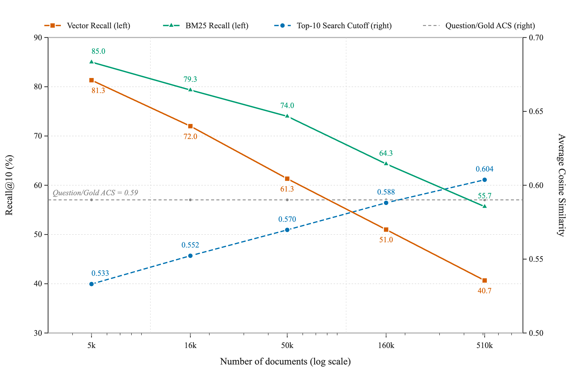
We start by only considering the EnterpriseRAG corpus. Specifically we split it into random samples that are added progressively to the gold documents, simulating a corpus that grows homogeneously. As we scale from 5k to 510k, vector recall@10 slides from 81% to 41% and BM25 from 85% to 56%. It is instructive to track the average cosine similarities for both, the cutoff for the top 10 and also the question and the gold-chunk comparison. The intuition is nicely confirmed: recall@10 drops below 50% as the average cutoff rises above the bar.

Figure 1: Recall@10 for BM25 and vector search both decline as the corpus grows from 5k to 510k, while the cosine score needed to reach the top 10 rises and crosses the typical question-to-answer similarity around 0.59 --- the moment most answers slip below the cutoff.

This curve is very consistent with the S-shape pattern for the recall curve discussed in the framework section. Since recall is bound by 1 and 0, the recall curve must flatten out on both ends. The length of the near-linear drop as a function of $\ln N$ is in fact rather striking. As we stated above, the drop depends on the distribution of the difficulty of the questions. The generation of the questions for the EnterpriseRAG benchmark certainly did not incorporate a mechanism for that, so one may wonder whether this behavior is fairly common. (Note that the recall results differ from Sun et al (2026) as we look here at a more difficult subset of questions.)

The k/N-dependence of recall. If we plot the observed recall for various $k$ as a function of $\ln N$ we see the expected behavior of recall declining for larger $N$ and smaller k:

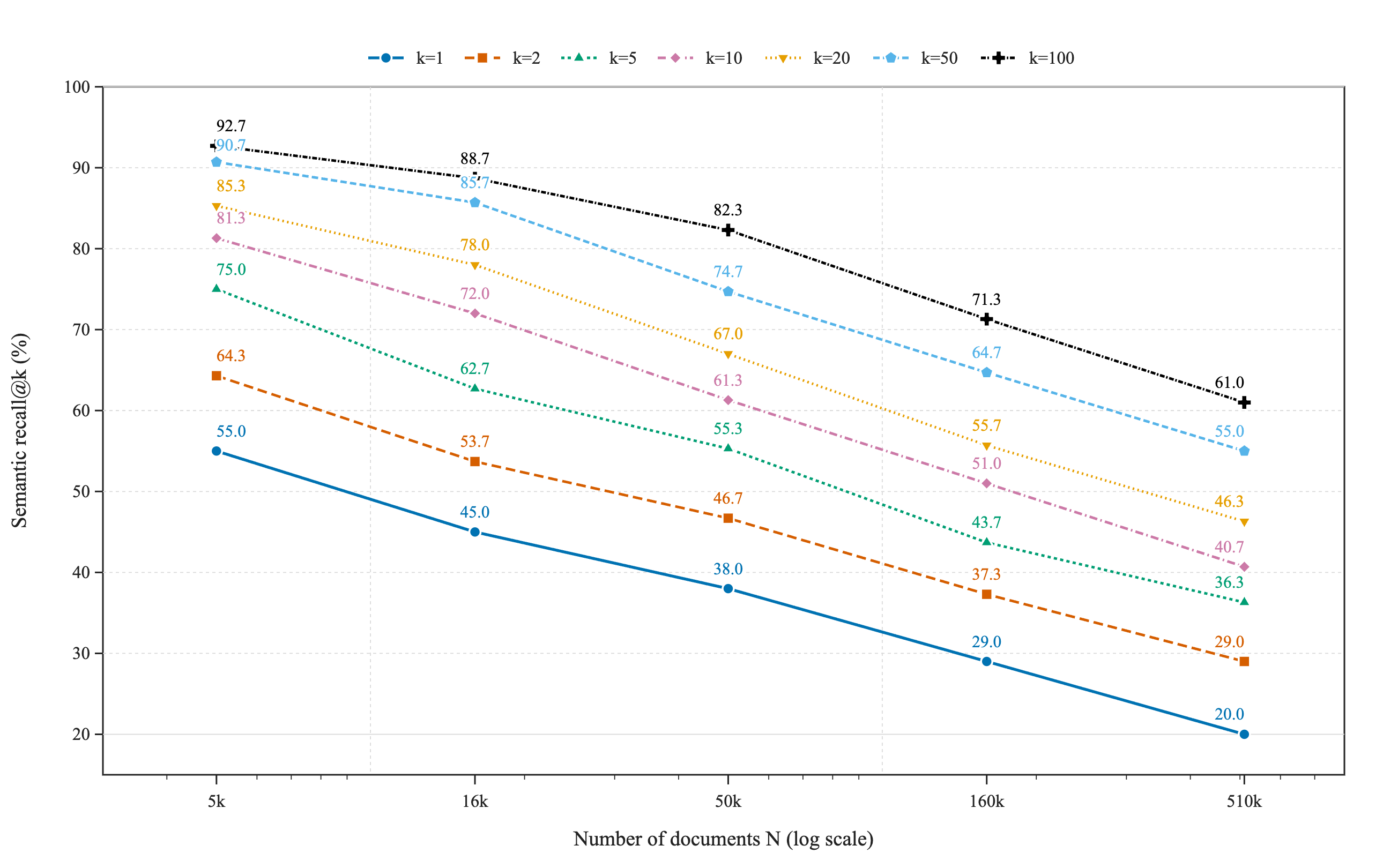
Figure 2: Vector recall@k versus corpus size for $k$ from 1 to 100: every curve declines as expected

The claim was that the recall curve only depends on k/N. If that is truly the case we should be able to predict recall at higher scale through the recall values at lower scale for lower k.

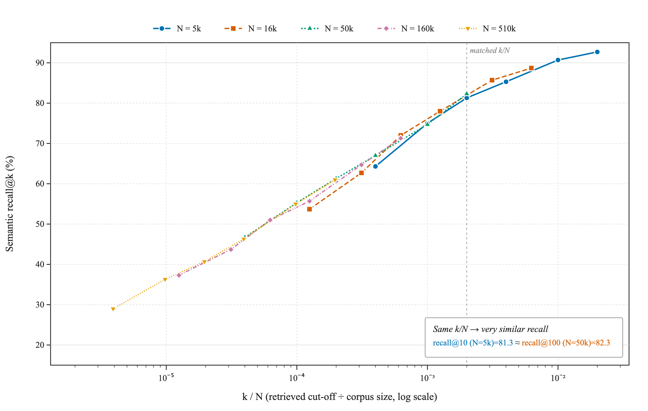
Or, equivalently, if we plot recall as a function of k/N, then the all curves that are distinct in Figure 2 should merge - recall at $k=2$ and $N=50$k should be very close to $k=20$ and $N=500$k.

And this is precisely what we see for both semantic and BM25 searches, as shown in Figure 3.

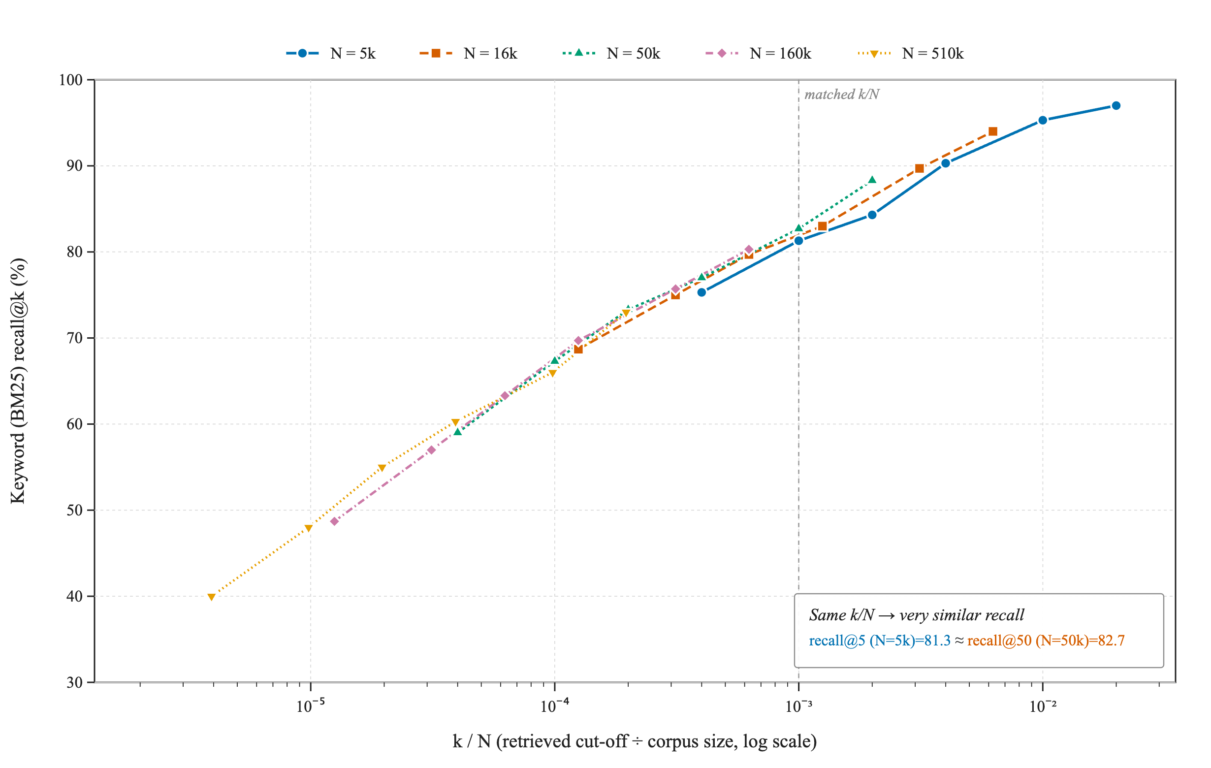
Figure 3: Semantic (left) and BM25 (right) recall@$k$ versus $k/N$ - confirming that the dependence is on $k/N$, not on $k$ and $N$ separately. $k=1$ was removed

3.2. Test 2: scaling with similar vs less similar documents

We saw the drop in recall for in-distribution scaling. We will now compare this behavior to documents that are not part of the same distribution. Specifically, we consider comparing scaling to 16k documents now to scaling by i) a biased subset of the EnterpriseRAG dataset and ii) a subset of the BrowseComp-Plus set, all with the same number of chunks.

We first consider the similarity test for the three extension sets of ~32k chunks corresponding to 11k EnterpriseRAG documents:

Random subset of EnterpriseRAG:

• $S_{AA} \sim S_{BB} \sim S_{AB} \sim 0.47$
• $\mathrm{MMD}^2(A, B) = S_{AA} + S_{BB} - 2\, S_{AB} \sim 0$

Biased subset of EnterpriseRAG:

• $S_{AA} \sim 0.47$
• $S_{BB} \sim 0.64$
• $S_{AB} \sim 0.53$
• $\mathrm{MMD}^2(A, B) \sim 0.05$

Random subset of BrowseComp-Plus:

• $S_{AA} \sim 0.47$
• $S_{BB} \sim 0.17$
• $S_{AB} \sim 0.18$
• $\mathrm{MMD}^2(A, B) \sim 0.28$

Based on these similarities, particularly also the low $S_{AB} \sim 0.18$ cross-similarity between EnterpriseRAG and BrowseComp-Plus documents, we anticipate hardly any impact on recall behavior for Enterprise RAG questions when we add BrowseComp-Plus documents.

The biased EnterpriseRAG subset seems to be located in a fairly tight subspace of the larger EnterpriseRAG distribution and has a higher degree of similarity with the main corpus. Correspondingly, we could likely expect some impact but less so than we would expect for the random EnterpriseRAG documents.

This is precisely what we see in Figure 4.

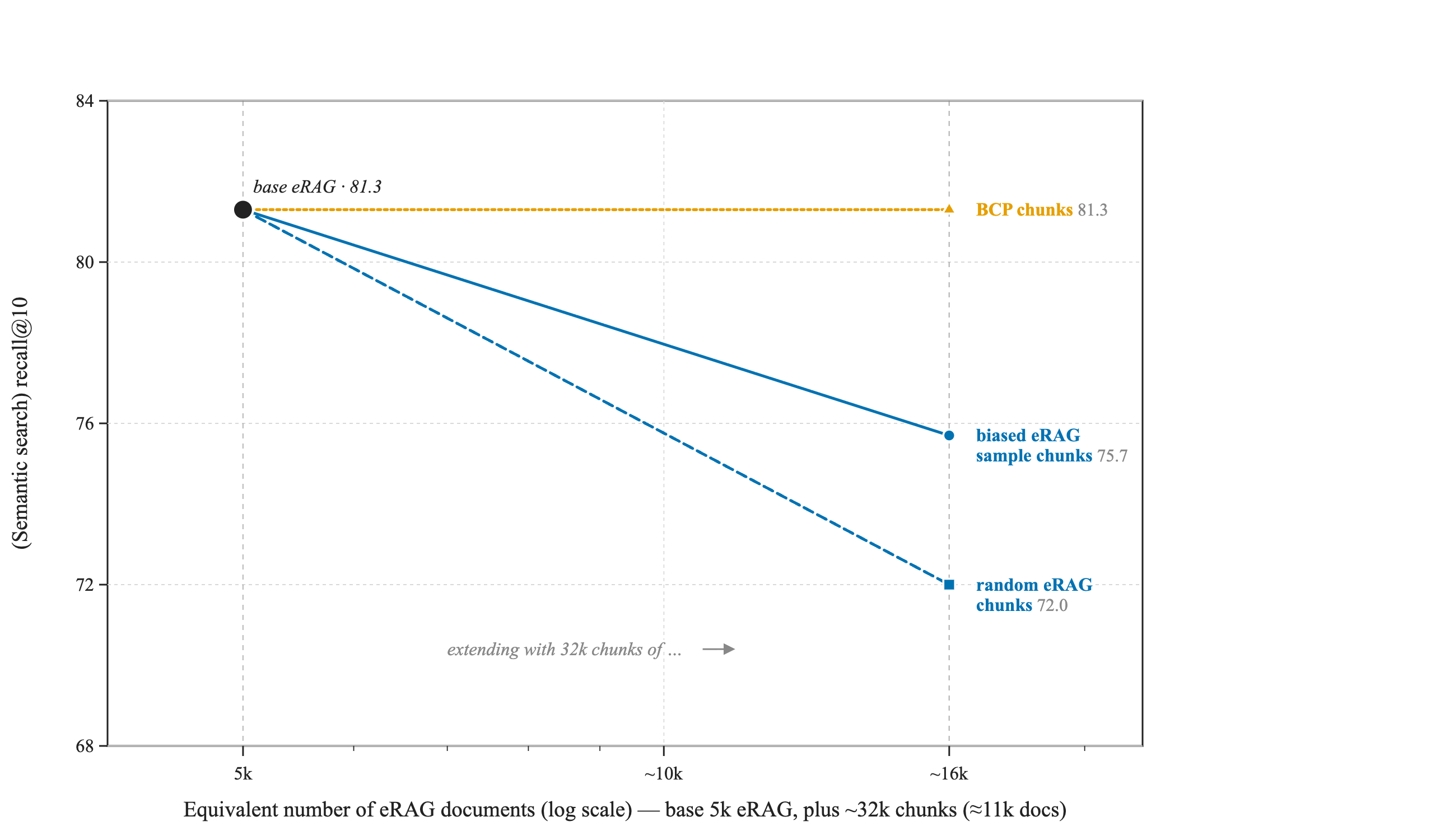
Figure 4: With the number of added documents held fixed, semantic recall@10 does not move for the strongly dissimilar additions from BrowseComp-Plus, but drops for similar ones --- as expected, overlap, not volume, is what hurts.

This result may be surprising at first sight as the biased eRAG sample is actually more similar to the average eRAG document, however they also occupy a substantially smaller volume in the semantic space and may well interfere heavily with some questions but be very far away from others.

That is precisely the gap between bulk similarity and per-question proximity. Here is a likely scenario: a random eRAG sample spreads across the whole distribution and competes a little with nearly every question; the biased sample crowds one tight region - hammering the handful of questions that live there and leaving the rest untouched. But averaged over all questions, it does less damage, even though it sits closer to your documents on average. Which is exactly why the $\mathrm{MMD}^2$ check is only a first screen and the per-question competition discount is the sharper tool: what governs recall is how close $B$ lands to your questions' answers, not its average similarity to your corpus.

Adding the whole BrowseComp-Plus corpus (100k documents) changes semantic recall@10 little, as seen in Figure 5.

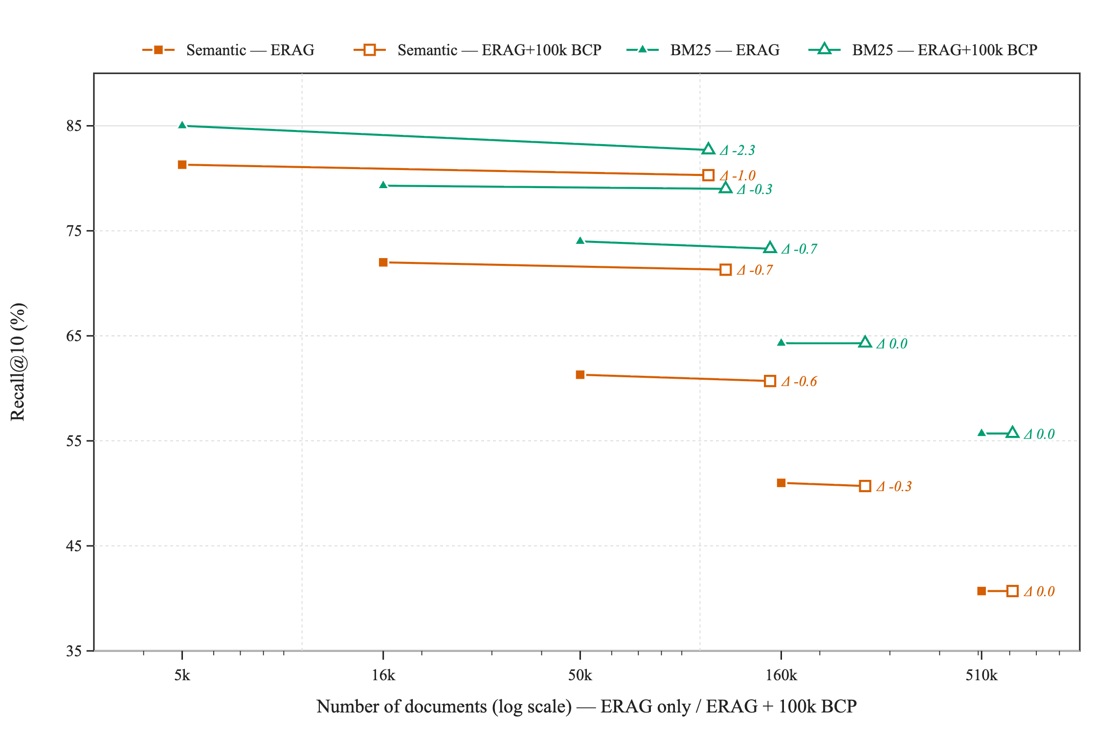
Figure 5: Adding 100k dissimilar BCP documents to the base corpus recall@10 changes little for both vector and keyword search --- out-of-distribution growth does almost no (or very small) damage.

Note that despite the high average distance, adding ~1.5m distracting chunks belonging to the 100k BrowseComp-Plus documents to the ~15k chunks from the 5k initial EnterpriseRAG set does have a small but non-zero impact on recall@10 - it falls by 1 percentage point for semantic search.

Making "far enough" precise is ultimately a question of geometry: how densely documents pack around a question depends on the effective (intrinsic) dimensionality of the embedding space, not its nominal coordinate count, and that geometry governs how fast competitors accumulate and how quickly the retrieval threshold climbs (Levina & Bickel, 2004; Li, 2011). We saw some intriguing behavior on this front in our own corpora that we hope to study further and write about separately.

3.3. Test 3: recall predictions via sampling

Finally, we applied the sampling-based prediction proposal to the EnterpriseRAG set. Specifically, we do that by simulating scaling up from 5k documents using i) the biased eRAG set leading to the equivalent of 16k documents, and ii) incrementally growing by adding random subsets of EnterpriseRAG to sizes 16k, 50k, 160k, and 510k.

All tests are done using the initial 5k data plus a 10% subset of the add-on set. And the predictions using the formalism work quite well as shown in Figure 6.

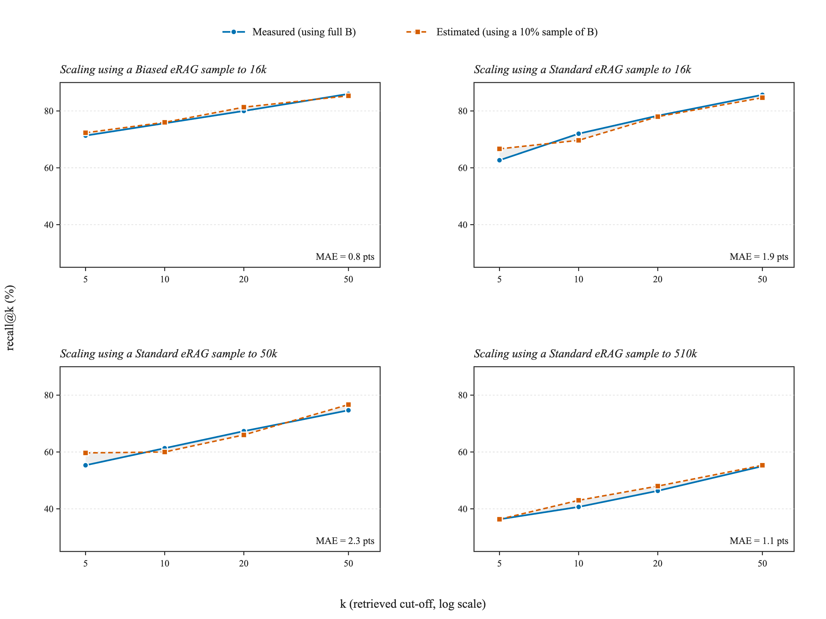
Figure 6: Predicted and estimated semantic recall at various $k$ using 5k documents + a 10% sample of the respective extension set - by size of the scale-up corpus.

If we compare the individual predictions across all scaling scenarios we arrive at Figure 7 which tells a very similar story. (We remove the case $k=1$ here as that is really a corner case.)

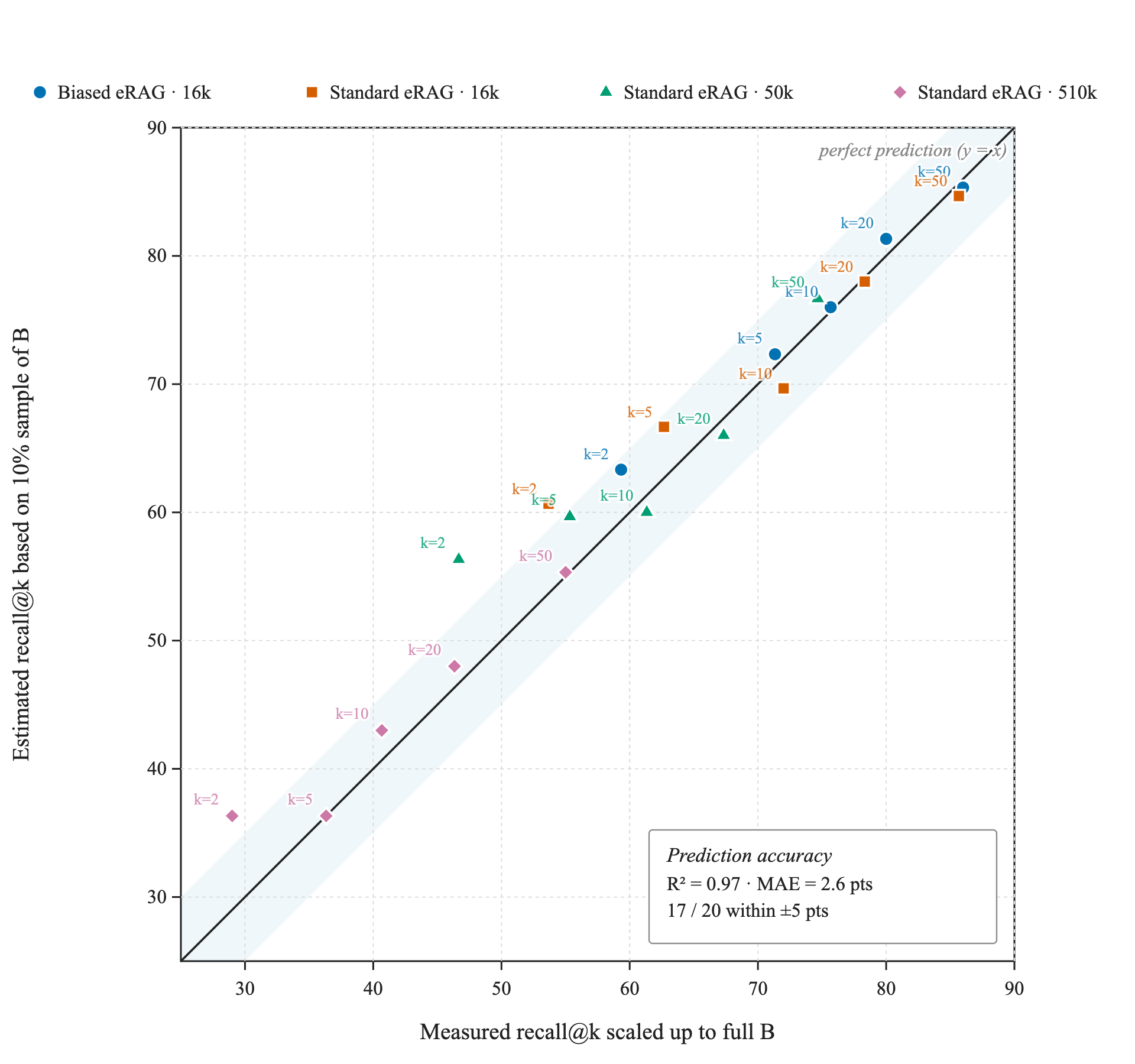
Figure 7: Predicted vs estimated semantic recall across all scaling sizes

3.4. Comments on keyword (BM25) and file search

This piece is about semantic search, but a short detour on keyword (BM25) search is worth it as we showed some results anyway.

One of the more striking features of the scaling data is that BM25 keyword search consistently beats semantic search at every scale, yet declines - within their linear range - along a nearly identical slope - and it actually degrades a touch more gracefully (Recall@10 falls 85.0% → 55.7% for BM25 vs. 81.3% → 40.7% for dense across the same 100× scaling). Both facts are illuminating, and both point toward the hybrid approaches in Part II.

Why BM25 wins on level. Even our "semantic" question category - written specifically to minimize keyword overlap - retains irreducible specific tokens. A question about EC2 instances in us-east-1 can't be rephrased without the region code; a question about a project deadline can't avoid the date. BM25 exploits these: us-east-1 is rare and strongly discriminative, earns a high IDF weight, and dominates the score when a document matches it exactly.

Semantic search treats the same tokens very differently. Current embedding models encode us-east-1 and us-west-2 as nearly interchangeable - both AWS regions, near-identical contexts - so the embedding distance between "how many instances in us-east-1" and "...in us-west-2" is tiny. Documents about the wrong region are barely penalized in vector space, and if many documents discuss us-west-2 and only one discusses us-east-1, the correct document is easily crowded out by its semantically near-identical but factually wrong neighbors. This recurs across high-specificity tokens generally - dates, version numbers, geographic identifiers, SKUs, internal project codes, person names. These are hard constraints (a correct retrieval must match them), but embedding models treat them as soft signals, flattening the distinction between the exact value and its near-synonyms. This isn't specific to text-embedding-3-small; it's a general property of how current embedding models handle high-specificity tokens.

Why the slopes nonetheless match. The underlying challenge is the same in both spaces: as an in-distribution corpus grows, documents about similar topics use similar words, so a rare discriminator stops being rare. At 5k documents us-east-1 might appear a handful of times; at 510k documents from the same enterprise distribution it appears in dozens or hundreds - infrastructure reports, cost analyses, postmortems, capacity plans - and BM25 must lean on ever-subtler combinations of term frequencies. The keyword space crowds the same way the embedding space does, because both reflect the same reality: more in-distribution documents means more documents that share the discriminative features, whether those features are embedding directions or terms.

So the two fail in different ways - vector misses exact constraints, keyword misses paraphrases and concepts - and their blind spots don't overlap. That non-overlap is exactly the opening the agentic strategies in Part II exploit. For the rest of this post, the protagonist stays semantic search.

What about file search? File search has recently become popular in solutions like Claude Code, Claude Cowork, OpenClaw, etc. as a method to retrieve information from a corpus for a larger agentic flow. Since it is de facto always part of an agentic flow we do not directly compare it here to BM25 or semantic search. However, we studied its scaling property in more detail in the blog "Are File Systems All You Need? It Depends..." and found that at scale it breaks down. And the reason is pretty clear - file search works similar to BM25 search but without the essential benefit of ranking, and the corresponding failure mode is very different and more severe: while BM25 may slowly lose the proper documents as the corpus size increases when their rank is pushed below k, file search relies to a good extent on filtered grep operations where the corpus is searched for keyword combinations and all results are returned - unranked! At some point the returned results are too large for an LLM to process and the searches are redone with higher specification. However, that often leads to substantial narrowing of the search and the proper documents are not retrieved anymore. The point is that this behavior is not expected to be a particularly smooth process and retrieval degradation is expected to look quite differently - first, within an agentic flow, the performance is expected to stay quite constant as nothing is missed; but at a certain scale the search narrowing occurs to maintain reasonable context to review and the retrieval quality should drop significantly, as observed in that blog.

---

4. What to take away

The through-line is the one we opened with: recall tracks $k/N$, not corpus size by itself, so widen the net as you grow; where you grow matters more than how much, since more of your most-queried topics is the expensive kind of growth while a genuinely different source is nearly free; and you can see it coming - forecast the decay from sub-samples and screen a new corpus with the question-only merge gate, both before you commit to a full index. And because semantic and BM25 fail in different ways, use them together in a hybrid.

For agentic search specifically, the framework and observations point to three tuning knobs:

• Increase $k$ efficiently. To scale a similar corpus by, say, 50×, increasing $k$ by 50× should largely hold recall — but it can blow up the LLM's context from ~5k to ~250k tokens. Parallelizing queries and using a cheaper model to pre-screen the returned chunks (passing only the promising ones to the main flow) keeps the cost down.
• Query more keyword combinations. Let the agent issue more keyword searches — and track which earlier searches came up empty, so it doesn't repeat ineffective ones.
• Consider ‘filtered semantic search’. Run a semantic search over a subset of documents constrained to contain keywords the model believes must appear verbatim.

Part II will pick up the obvious next question: if plain retrieval decays this predictably, can a smarter, agentic search strategy - one that iterates, combines keyword and vector search, and uses these very diagnostics to steer itself - win back what scale takes away? It can. More soon.

---

Acknowledgements

We enjoyed interesting and helpful conversations with Mark Butler.

References

None of the ideas here is new on its own - the value, if there is any, is in pulling them together. That spread is worth seeing laid out, because it's why no single prior source answers the practical question: the pieces come from keyword-era IR, signal-detection statistics, manifold learning, and a few 2024–2025 RAG papers, and they don't normally appear in the same room.

Collection size and retrieval effectiveness

• Hawking, D. & Robertson, S. (2003). On Collection Size and Retrieval Effectiveness. Information Retrieval 6(1), 99–105. - The original "retrieval gets harder as the collection grows," for keyword search.
• Madigan, D., Vardi, Y. & Weissman, I. (2006). Extreme Value Theory Applied to Document Retrieval from Large Collections. Information Retrieval 9(3), 273–294. - Heavy-tailed score modeling at scale.

Score distributions and query performance prediction (predicting effectiveness without labels)

• Manmatha, R., Rath, T. & Feng, F. (2001). Modeling Score Distributions for Combining the Outputs of Search Engines. SIGIR '01: Proceedings of the 24th Annual International ACM SIGIR Conference on Research and Development in Information Retrieval, 267–275. - The score-distribution view that the survival-function model rests on.
• Kanoulas, E., Pavlu, V., Dai, K. & Aslam, J. (2010). Modeling the Score Distributions of Relevant and Non-relevant Documents. SIGIR '10: Proceedings of the 33rd International ACM SIGIR Conference on Research and Development in Information Retrieval, Geneva, Switzerland, July 19–23, 2010.
• Vlachou, M. & Macdonald, C. (2024). Coherence-based Query Performance Measures for Dense Retrieval. ICTIR (arXiv:2310.11405). - Query performance prediction carried over to dense retrievers.

The similarity / merge-gate machinery

• Gretton, A., Borgwardt, K., Rasch, M., Schölkopf, B. & Smola, A. (2012). A Kernel Two-Sample Test. JMLR 13, 723–773. - Maximum Mean Discrepancy; the $S_{AA} + S_{BB} − 2 \cdot S_{AB}$ statistic behind the near/far check.
• Webber, W. (2013). Approximate Recall Confidence Intervals. ACM Transactions on Information Systems (TOIS) 31(1), Article 2, 1–33. - Putting error bars on recall estimated from a sample; the statistics behind forecasting from a B-sample.

Dense vs. sparse at scale

• Reimers, N. & Gurevych, I. (2021). The Curse of Dense Low-Dimensional Information Retrieval for Large Index Sizes. Proceedings of the 59th Annual Meeting of the Association for Computational Linguistics and the 11th International Joint Conference on Natural Language Processing (Volume 2: Short Papers) (arXiv:2012.14210). - Why dense retrieval degrades faster than sparse as the index grows.

Corpus scaling in RAG (the coverage side, and what not to confuse this with)

• Ning, J., Kong, Y., Long, Y. & Callan, J. (2025). Less LLM, More Documents: Searching for Improved RAG. Advances in Information Retrieval: 48th European Conference on Information Retrieval, ECIR 2026, Delft, The Netherlands, March 29–April 2, 2026, Proceedings, Part I (arXiv:2510.02657). - A bigger corpus can improve end-to-end RAG by covering more answers; the coverage effect we contrast against the competition effect.
• Levy, S., Mazor, N., Shalmon, L., Hassid, M. & Stanovsky, G. (2025). More Documents, Same Length: Isolating the Challenge of Multiple Documents in RAG. Findings of the Association for Computational Linguistics: EMNLP 2025, 19539–19547, Suzhou, China (arXiv:2503.04388). - More retrieved documents at fixed context can hurt the generator - a different axis from corpus size.
• Fang, Y. et al. (2024). Scaling Laws for Dense Retrieval. SIGIR (arXiv:2403.18684). - Scaling of model and training-data size, not corpus size; included to mark the distinction.

Effective (intrinsic) dimension of embeddings

• Levina, E. & Bickel, P. (2004). Maximum Likelihood Estimation of Intrinsic Dimension. Advances in Neural Information Processing Systems 17 (NIPS 2004). - Why embeddings behave as if they live in far fewer dimensions than their coordinate count, which sets how fast the retrieval threshold climbs.
• Li, S. (2011). Concise Formulas for the Area and Volume of a Hyperspherical Cap. Asian Journal of Mathematics and Statistics 4(1), 66–70. - The geometry behind counting near-neighbors on the sphere.

Benchmarks and Corpora

• Sun, Y. et al. (2026). EnterpriseRAG-Bench: A RAG Benchmark for Company Internal Knowledge. (arXiv:2605.05253)
• Chen, Z. et al. (2025). BrowseComp-Plus: A More Fair and Transparent Evaluation Benchmark of Deep-Research Agent. (arXiv:2508.06600)